23 July 2021: Clinical Research
Evaluation of Sanders Type 2 Joint Depression Calcaneal Fractures in 197 Patients from a Single Center Using Three-Dimensional Mapping
Xiaobo Guo1ABCDEF*, Xiaonan Liang2AB, Jiangtao Jin1D, Jinwei Chen1EF, Junyang Liu3B, Jinming Zhao4ABCDEFDOI: 10.12659/MSM.932748
Med Sci Monit 2021; 27:e932748


Abstract
BACKGROUND: This study aimed to evaluate Sanders type 2 calcaneal fractures in 197 patients from a single center using the 3D (three-dimensional) CT (computed tomography) mapping method.
MATERIAL AND METHODS: A consecutive series of 197 Sanders type 2 joint depression calcaneal fractures was used. The segment and split functions were used to create each calcaneal fragment using Mimics Research 20.0 software. The fracture fragments were reduced in 3-matic Research 12.0 software. In the E-3D Medical 18.01 software, after superimposing the fractured calcaneus entity with the calcaneus template, we drew the fracture line on the template. Finally, the heatmap was obtained by fracture statistical analysis function. Simultaneously, the distribution of the fracture lines in the anterior part of the calcaneus (APC) and middle talar joint was recorded.
RESULTS: There were 109 cases of Sanders type 2A, 46 cases of Sanders type 2B, and 42 cases of Sanders type 2C. Based on the data, we drew the characteristic fracture map of type 2A 2B and 2C. This study found that the most common types of Sanders type 2A in APC and middle talar articular surface are type AC and type AD. In Sanders type 2B, the most common type is type AC, and in Sanders type 2C it is type ACD.
CONCLUSIONS: The findings from this study showed that 3D CT imaging and reconstruction of the calcaneus was a useful diagnostic method to evaluate and classify joint depression calcaneal fractures. The calcaneal fracture map can be used to guide surgical planning and optimize the design of internal fixation.
Keywords: Calcaneus, Tomography, X-Ray Computed, Imaging, Three-Dimensional, intra-articular fractures, Diagnosis, Adolescent, Aged, 80 and over, Fractures, Bone, young adult
Background
The calcaneus is the largest tarsal bone in the foot, and it plays an important role in weight-bearing and walking [1,2]. It has been reported in the literature that 75% of calcaneal fractures are intra-articular fractures [3]. Accurate and timely classification of calcaneal fractures and estimating the shape of the fracture fragments are of great significance.
In recent years, increased attention has been paid to the surgical treatment of intra-articular calcaneal fractures because accurate posterior facet reduction can lower the incidence of traumatic arthritis of the subtalar joint [4]. Most calcaneal fractures are comminuted fractures, but each subtype has a unique fracture line distribution. The Essex-Lopresti classification [5] was proposed in 1952, which is based on X-rays. Calcaneal fractures can be divided into 2 types, tongue-like and joint depression fracture. These fractures can be further divided into 3 types based on the degree of displacement. The Essex-Lopresti classification evaluates the general displacement of calcaneal fractures [5]. The Essex-Lopresti classification is simple and convenient, but it cannot accurately judge the injury of the articular surface of the calcaneus. The Sanders classification [6] is based on computed tomography (CT) images. Sanders type 2 calcaneal fractures are divided into type 2.a, which involves the lateral aspect of the posterior facet; type 2.b, which involves the central aspect of the posterior facet; and type 2.c, which involves the medial aspect of the posterior facet, with a transverse fracture of the body of the calcaneus [6]. Nonetheless, the Sanders classification is only based on the posterior subtalar articular surface of the calcaneus, which cannot fully describe the whole fracture line distribution. The anterior part of the calcaneus (APC) is an important part of the calcaneus, but there are few reports on the fracture line distribution of the APC. With the development of picture archiving and communication system (PACS) and CT technology, it is possible to extract three-dimensional (3D) data of the calcaneus, which can comprehensively guide our understanding and surgical treatment of calcaneal fractures [7,8].
The fracture map is also called the fracture line distribution map, which was first proposed in 2009 by Armitage et al [9]. The three-dimensional fracture entity is reconstructed by computer software, the fracture lines of multiple cases are superimposed on a standard model, and a heatmap or frequency map is used to analyze the distribution of the fracture line to describe the start and end, direction, distribution, and fracture of the fracture line shattered situation. The fracture map helps orthopedists analyze the characteristics of fractures more three-dimensionally, and guide the design of medial fixation and intraoperative reduction more effectively. Ni et al [10] used CT data of 62 patients with complex calcaneal fractures to draw a map of complex intra-articular calcaneal fractures. However, the calcaneus has a variety of injury mechanisms that cause different types of fractures, which need to be further explored. Therefore, this study aimed to evaluate the fracture lines distribution of Sanders type 2 joint compression calcaneal fractures in 197 patients from a single center using 3D-CT, thereby providing a reference for clinical treatment.
Material and Methods
PATIENT COHORT:
This study was approved by the Ethics Committee of Jincheng General Hospital, and was conducted in accordance with the declaration of Helsinki (No. 20200901). From January 2013 to December 2021, 197 cases of Sanders type 2 joint depression calcaneal fractures were selected. The inclusion criteria were as follows: (1) Age 18–80 years, (2) Availability of complete X-ray and CT scan data, and (3) Closed fracture of the calcaneus. The exclusion criteria were as follows: (1) Comminuted fracture and difficulty in confirming the fracture line, (2) CT does not meet the requirements and the image quality is poor, and (3) Pathological and osteoporotic fractures (Table 1).
CT DATA ACQUISITION AND 3D RECONSTRUCTION:
All 197 patients underwent Siemens 64 slice spiral CT (120 kV, 350 MA, slice thickness 0.75 mm), and a healthy volunteer (male, 30 years old, 170 cm tall, signed informed consent) was selected as the template. The scan data in digital imaging and communications in medicine (DICOM) format were imported into Mimics Research 20.0 (Materialise, Leuven, Belgium) software. According to Sanders classification, the calcaneal fractures were categorized into Sanders type 2A, type 2B, and type 2C. Initially, the sagittal view of the CT images was selected in the Mimics software, the bone threshold was chosen, and the mask of all ankles was generated. Subsequently, the split mask function was used to separate the calcaneus from the other bones. Next, the split mask function was applied to separate the calcaneus fragments again (Figure 1A). The separated fragments were imported into the 3-matic Research 12.0 (Materialise, Leuven, Belgium) software, and the fracture fragments were repositioned by rotation and translation. Finally, the 3D entity of the calcaneus after reduction was obtained as the output (Figure 1B).
CONSTRUCTION OF THE 3D FRACTURE MAP:
The 3D entity of the calcaneus after reduction was imported into E-3D Medical 18.01 (Central South University, Changsha, China) software. The 3D entity of the calcaneus was registered with the template calcaneal entity, and it is was completely coincident with the standard entity by rotation, scaling, and overlapping of the landmark points. After registration, the fracture line of the calcaneus was drawn in the 3D image of the calcaneal template. The same operation was performed with all 197 cases. The fracture heatmap function was employed to convert the calcaneal fracture lines into the heatmap. The transformation was based on the frequency of the calcaneal fracture line in each position of the 3D template. The area within 2 mm of the fracture line was defined as the fracture line area. The closer the fracture line, the higher the weight (Figure 1C). The 3D fracture map method used in this study is based on the previously described method [10–12]. The general and Sanders type 2A, type 2B, and type 2C of joint compression calcaneal fractures followed the above methods. Then, the superimposed picture and heatmap of the fracture line on the calcaneal template were exported in the standard top, bottom, lateral, medial, front, and rear views.
DATA COLLECTION:
The Sanders type 2A, type 2B, and type 2C calcaneal fractures were counted according to the axial CT images. Two professional foot and ankle surgeons performed the classification independently and compared them after completion. Discuss and consult the third researcher when the classification is inconsistent. Subsequently, the APC was divided into A, B, and C zones from the lateral to the medial. The middle subtalar articular surface was considered as the D zone. The frequency of each fracture in a specific area was determined (Figure 2).
Finally, the 3D concentration trend and the distribution of calcaneal fracture lines of Sanders type 2A, type 2B, and type 2C were observed in a multidirectional orientation. In the E3D software, internal fixation planning function was applied to plan the talar articular surface screw placement position. Multidirectional analyses repeatedly confirmed that the screw was fixed in the intact bone. Next, we recorded and described the screw position.
STATISTICAL ANALYSIS:
Statistical Product and Service Solutions (SPSS) software v.26.0 (IBM, Inc., Armonk, NY, USA) was used for data processing. Continuity data are expressed using mean and standard deviation. Count data are represented by frequency and percentage. In fracture distribution in APC and middle talar articular surface, all cases were divided into 3 groups (Sanders type 2A, 2B, and 2C) for analysis. The chi-square or Fisher exact test was used to analyze the differences between groups, and P<0.05 was considered statistically significant.
Results
GENERAL JOINT DEPRESSION 3D MAP CHARACTERISTIC:
In the top view, the 2 concentration areas respectively appeared from the medial and lateral portions of the middle-third region of the calcaneal body. The concentration areas converged forward, passed through the lateral third region of the posterior talar articular surface, and reached the intersection of the APC and the posterior talar articular surface. Next, the line was divided into 3 branches, and the first branch was located at the lateral part of APC. The second branch was situated in the transitional part of the APC and the middle talar articular surface. The third branch was present in the middle of the middle talar articular surface. The first and second branches ran forward and down to the sole, while the third branch ran inward to the sole. In the lateral view, 2 longitudinal fracture concentration areas were present on the lateral surface; one was located in the transitional area of the lateral surface and the posterior surface of the calcaneus, and the other one was the origin in the tip of GA and extended backward. These 2 concentration areas were arc-connected at the posterior part of the lateral surface. One oblique line originated in the tip of the GA and ran obliquely to the sole. In the medial view, the fracture line ran along the middle part of the calcaneus obliquely downward and forward. This line was divided into 2 branches, one ran longitudinally forward in the medial-middle portion of the calcaneus, while the other run downward to the sole. The concentration areas of the calcaneocuboid articular surface were concentrated in the lateral and medial thirds. From the bottom view, it was evident that the concentration areas were concentrated in the front and back third portions (Figures 3, 4).
SANDERS TYPE 2A JOINT DEPRESSION 3D MAP CHARACTERISTIC:
In the top view, it was evident that the 2 arc-shaped concentration areas appeared in the medial and lateral of calcaneus body and coincided in the lateral third portion of the posterior talar articular surface, which was consistent with the general view. The concentration areas moved obliquely forward and downward through the lateral third region of the posterior talar articular surface, running longitudinally to the lateral and medial regions of the APC, respectively. Meanwhile, the other concentration areas also ran transversely to the middle part of the middle talar articular surface. The lateral, bottom, medial, and front views were consistent with the general view (Figures 5, 6).
SANDERS TYPE 2B JOINT DEPRESSION 3D MAP CHARACTERISTIC:
In the top view, we could see that the 2 arc-shaped concentration areas appeared in the dorsal calcaneal body and coincided in the middle third of the posterior talar articular surface. In comparison with the general view, the lateral arc seemed backward than general view, and the medial arc seemed forward than general view. They moved obliquely forward and downward through the middle third of the posterior talar articular surface, running longitudinally to the lateral and medial portions of the APC, respectively. The bottom, front, and lateral views were consistent with the general view. The medial view was the same as the general view, but was more forward and upward than the general view (Figures 7, 8).
SANDERS TYPE 2C JOINT DEPRESSION 3D MAP CHARACTERISTIC:
In the top view, it was evident that the 2 arc-shaped concentration areas appeared in the dorsal calcaneal body and coincided in the medial third portion of the posterior talar articular surface. In comparison with the general view, the lateral arc was backward, and the medial arc was more forward than Sanders type 2B. It moved obliquely forward and downward through the medial third of the posterior talar articular surface, running longitudinally to the lateral and medial portions of the APC, respectively. The bottom, front, and lateral views were consistent with the general view. The medial view was the same as the general view, but was more forward and upward than Sanders type 2B (Figures 9, 10).
FRACTURE DISTRIBUTION IN APC AND MIDDLE TALAR ARTICULAR SURFACE:
The proportions of Sanders type 2A, 2B, and 2C involved in area A were 84.4%, 87%, and 90.5%, respectively, and there was no statistically significant difference between the 3 groups. The B area involved in the 3 groups was less than or equal to 23.9%, and there was no statistically significant difference among them. The proportions of Sanders type 2A, 2B, and 2C involved in area C were 48.6%, 73.9%, 66.7%, respectively, and the proportion of Sanders type 2B and 2C was significantly higher than type 2A. The proportions of Sanders type 2A, 2B, and 2C involved in area D were 50.5%, 15.2%, 73.8%, respectively, and the proportion of Sanders type 2C was significantly higher than type 2A and 2B, and type 2A was significantly higher than type 2B.
In Sanders type 2A, the highest types were type AC (30.3%) and type AD (24.8%). In Sanders type 2B, the highest type is type AC (58.7%) and it was significantly higher than Sanders’s type 2A and 2C. In Sanders type 2C, the highest type is type ACD (40.5%), and it was significantly higher than Sanders type 2A and 2B (Table 2).
Discussion
The shape of the calcaneus is complex, with several articular surfaces present in it. The integrity of its anatomical form is of great significance in maintaining the normal joint function of the hind foot, supporting the arch of the foot, and the stress transfer of the lower limb during loading. It is extremely important to restore the height, length, width, Bohler’s angle, and Gissane’s angle of the calcaneus, as well as the anatomical structure of the talar joint during calcaneal fracture surgery. The restoration of the posterior talar articular surface anatomy is closely related to the functional outcome, and articular incongruences >1 mm result in increased contact pressure, secondary arthritis, and inferior functional outcomes [6,13]. The reduction is challenging due to the complex geometry of the articular surface.
The conventional CT combined with 3D reconstruction technology improves the visual analysis of complex fractures. Considering that 3D-CT can better visualize the talar articular surface, it innovates the conventional understanding of the calcaneal fracture [14]. The use of 3D-CT can accurately evaluate the fracture line distribution, displacement direction, and the joint surface involvement to enable selection of the appropriate treatment approach and thereby the evaluation of the relevant prognosis more effectively. The 3D-CT technique has been widely used for preoperative planning and intraoperative reduction of calcaneal fractures [15,16]. In this study, the CT data of calcaneal fracture with 0.75-mm slice thickness were used for 3D reconstruction to accurately visualize the distribution of the calcaneal fracture line and the displacement of fracture fragments. Simultaneously, the split technology of the Mimics software was used to completely display the involvement and displacement of talar articular surface.
Fracture mapping technology, also known as fracture line distribution mapping, was first proposed in 2009 by the team in the Department of Orthopedics, University of Minnesota [9]. Fracture mapping is a method that superimposes the fracture lines of multiple fracture models on a normal model through CT 3D reconstruction in order to visually display the shape of the fracture. This technology directly reveals the morphological characteristics of the fracture line and provides a novel method for fracture diagnosis and classification, treatment scheme selection, internal fixation design, fracture prone site statistics, and fracture standardized model formulation. Fracture mapping technology has so far been applied to scapular [9], distal tibial [17], ulnar coronoid process [18], tibial plateau [19], radial head [20], intertrochanteric [21], Hoffa [12], acetabular [22,23], lumbar [11], posterior malleolus [24], and calcaneal fractures [10].
More than 60% of calcaneal fractures are caused by axial load after falling from a height [25–29]. In this study, 67.5% of the cases were caused by falling from a height. Several past studies have described the distribution of the fracture line and the displacement of fracture fragments in the calcaneus. For example, Essex-Lopresti indicated that the axial stress was transmitted to the calcaneus through the medial and lateral pathways through the tibia and talus. The posterior talar joint reversed and the taloid spur separated the calcaneal body from the lateral wall like an ax in the outer router. The inner router takes stress from the talar joint to the sustentaculum talus, splitting a portion of the posterior articular surface together with the sustentaculum tali with the calcaneal body. The secondary fracture line runs across the body immediately behind the talar joint. When the fracturing force continues, the joint fragment is depressed into the spongy bone of the body inside the lateral wall [5].
Regarding the mechanism of the calcaneal fracture occurrence, Teubner et al revealed that when the foot was in the dorsiflexion position, it was usually a tongue fracture, and when the foot was in the plantar flexion position, it was usually a joint depression fracture [30]. Zwipp et al suggested that when a person falls from a height, the heel lands in the entropion or valgus position, and the lateral edge of the talus cuts into the GA. Hence, the calcaneal fracture occurs in the medial or lateral side of the longitudinal axis. If the trauma continues, a fracture line passing through the posterior talar joint is produced [31]. This conclusion is similar to that of Badillo et al [14]. Tsubone et al used the finite element (FE) model to reveal that the fracture lines always started at the lateral side of the posterior articular fragment and extended along anteromedially to posterolaterally, while the other extended anterolaterally to posteromedially and behind the sustentaculum tali [32]. From the lateral view of the joint depression, it can be seen that the typical fracture area of the lateral wall and the middle of the lateral wall obliquely rupture due to the talus spur split. From the medial view, the typical fracture line where the sustentaculum tali is split can be displayed. From the top view, we can see the primary fracture line surrounding the sustentaculum tali and the secondary fracture line of joint depression fragment. From the rear view, we can see that none of the fracture lines pass through the calcaneal tuberosity (Figures 3, 4). Sanders type 2A, type 2B, and type 2C joint depression have their own distribution characteristics (Figures 5–10).
The APC is a saddle-shaped promontory at the anterior aspect of the calcaneus of varying length, breadth, and shape. It forms the anterior talar articular surface and the superior-posterior part of the calcaneal-cuboid articular surface. Most classifications for calcaneal fractures, such as the AO-Classification [33], the Essex-Lopresti classification [5], or the Sanders classification [6], either do not or only partially describe the APC fractures. This study found that the most common types of Sanders type 2A in APC and middle talar articular surface are type AC and type AD. In Sanders type 2B, the most common type is type AC and in Sanders type 2C it is type ACD. This result helps to improve the existing calcaneal fracture classification and further explain the injury mechanism of calcaneal fracture.
In the traditional CT 3D reconstruction images, due to the occlusion of the talus and cuboid, the upper and anterior surface of the calcaneus cannot be displayed, so the fractures of the talar joint and APC cannot be displayed. Veltman et al [34] believed that the addition of three-dimensional CT imaging did not increase inter- and intraobserver reliability for the classification of calcaneal fractures and commented they experienced no additional benefit from 3D-CT imaging for the assessment of calcaneal fractures. However, Veltman used a small sample of 38 cases. This study used 197 Sanders type 2 joint compression fractures for fracture mapping. In this study, through the split function of Mimics software, the calcaneus entity can be easily extracted from the ankle bone separately. Through this method, the surgeon can indirectly judge the distribution of the talar joint fracture line of the calcaneal joint depression fracture through Sanders classification by CT 2D images, thereby guiding the operation. Through the drawing of a fracture map, it can reflect the most common location of joint depression fracture line and the area not involved by the fracture line. Then, the internal fixation design can cross the fracture line while the screw is placed in the sparse area. Thereby, the fracture fixation is more stable and the probability of failure of the medial fixation is reduced at the same time.
Several screw trajectory methods are available for minimally invasive percutaneous screw fixation of the calcaneal fracture, and they depend on the fracture configurations [35]. The sustentaculum tali is one of the most important anatomical landmarks of the calcaneus. Owing to the constraints of the joint capsule and the surrounding ligaments and tendons, the sustentaculum tali is rarely displaced from the medial wall of the calcaneus [36]. Therefore, screws can be fixed from the lateral wall of the calcaneus to the sustentaculum tali to augment the implant stability [37]. It can be inferred from the calcaneus heatmap that for Sanders type 2A joint depression fracture, the intact bone area is mainly in the posterior part of the sustentaculum tali. Hence, the head of the screw meant for fixing the posterior talar articular surface should be located in the posterior part of the sustentaculum tali, and there was only one screw available (Figure 11A). For Sanders type 2B joint depression fracture, the bone of the sustentaculum tali is intact. Therefore, the head of the screw for fixing the posterior talar articular surface can be in any part of the sustentaculum tali, and there were several screws available (Figure 11B). For Sanders type 2C fractures, the bone in the medial surface of the posterior talar articular surface and the sustentaculum talus is insufficient. Thus, a plate should be used to fix the lateral part of posterior talar articular fragment (Figure 11C). In joint depression fractures, the fracture line of the APC is located in areas A and C; therefore, for the axial screw of the calcaneus, the tip of the screws should be located in area B (Figure 11D, 11E).
This study also has limitations. One of the limitations is the small sample size and the use of a single center; therefore, the bias that may be introduced. The other limitation is that a new classification system has not been established. Furthermore, whether the functional recovery of the joints can be predicted needs to be verified in future studies.
Conclusions
The findings from this study showed that 3D CT imaging and reconstruction of the calcaneus is a useful diagnostic method to evaluate and classify joint depression calcaneal fractures. The calcaneal fracture map can be used to guide surgical planning and optimize the design of internal fixation.
Figures
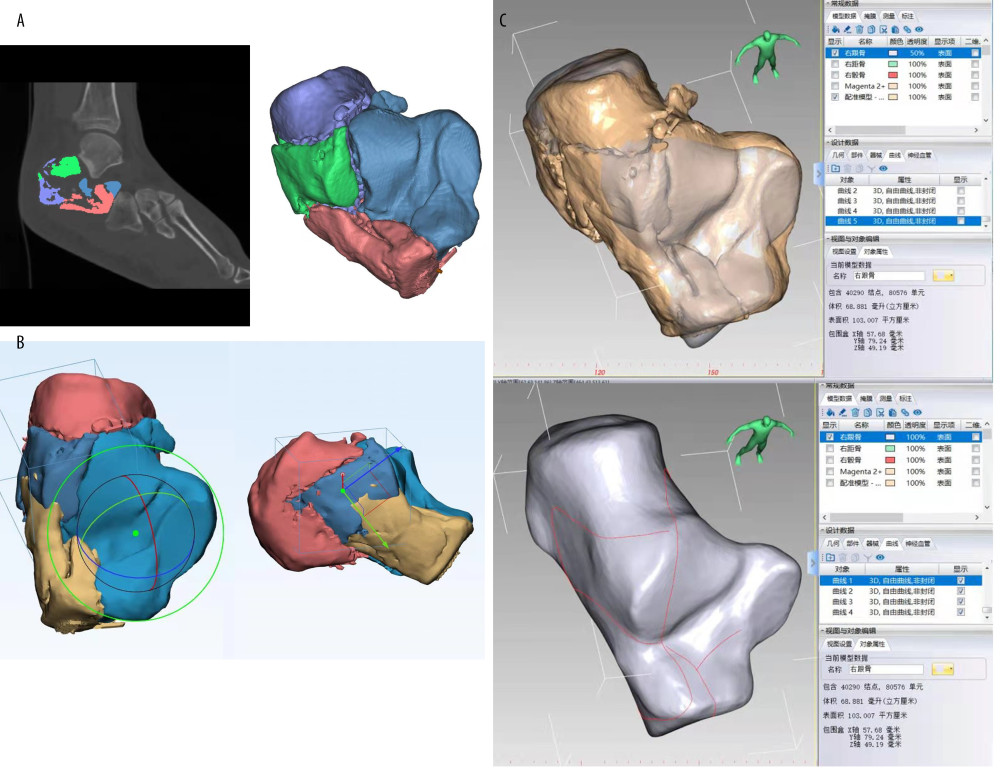 Figure 1. Flow charts of the calcaneal fracture map. (A) The segment and split functions were used to create each calcaneal fracture fragment by Mimics Research 20.0 (Materialise, Leuven, Belgium) software. (B) The calcaneal fracture fragments were reduced in 3-matic Research 12.0 (Materialise, Leuven, Belgium) software. (C) In the E-3D Medical 18.01(Central South University, Changsha, China) software, after superimposing the fractured calcaneus entity with the calcaneus template, draw the fracture line on the template.
 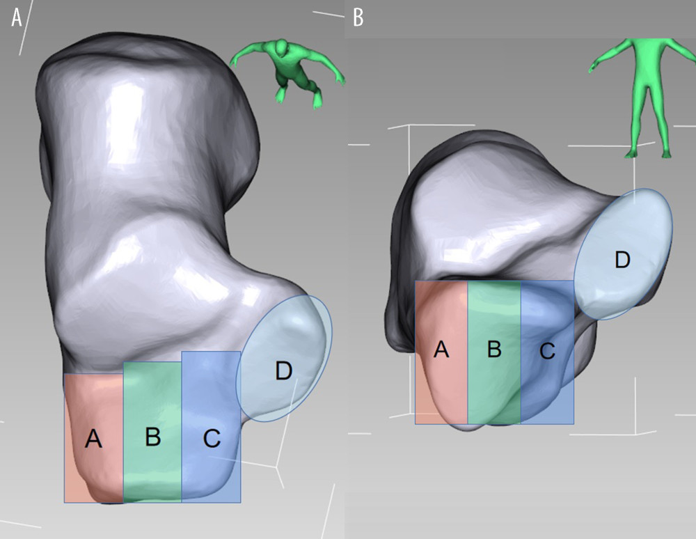 Figure 2. The division of the anterior part of calcaneus (APC) and middle talar articular surface. (A) Top view, (B) Front view.
 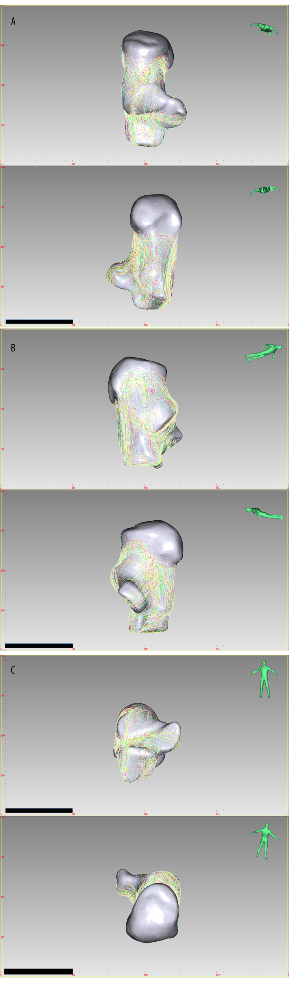 Figure 3. The fracture line distribution of Sanders type 2 joint depression fracture, created by E-3D Medical 18.01 software (Central South University, Changsha, China). (A) Top view, Bottom view, (B) Lateral view, Medial view, (C) Front view, Rear view.
 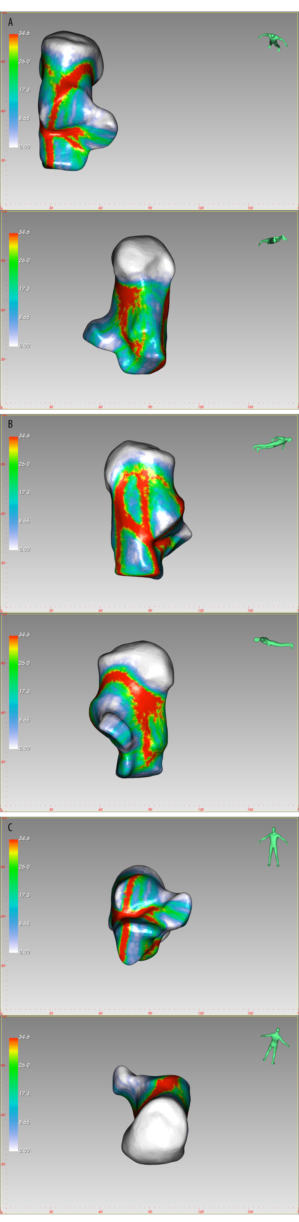 Figure 4. The fracture heatmap distribution of Sanders type 2 joint depression fracture, created by E-3D Medical 18.01 software (Central South University, Changsha, China). (A) Top view, Bottom view, (B) Lateral view, Medial view, (C) Front view, Rear view.
 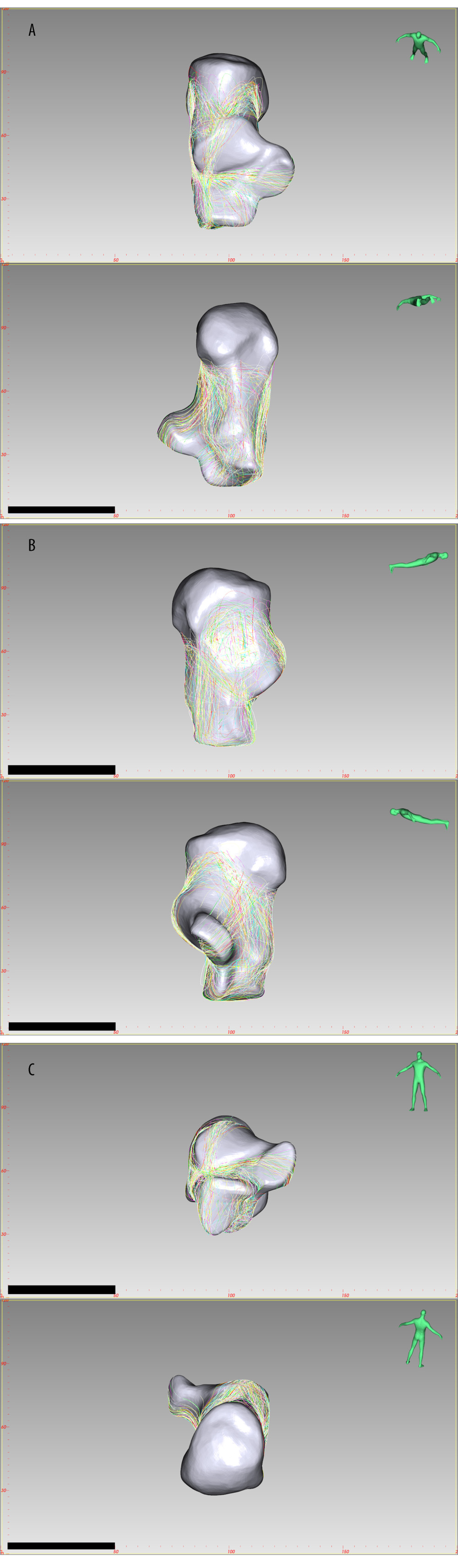 Figure 5. The fracture line distribution of Sanders type 2A joint depression fracture, created by E-3D Medical 18.01 software (Central South University, Changsha, China). (A) Top view, Bottom view, (B) Lateral view, Medial view, (C) Front view, Rear view.
 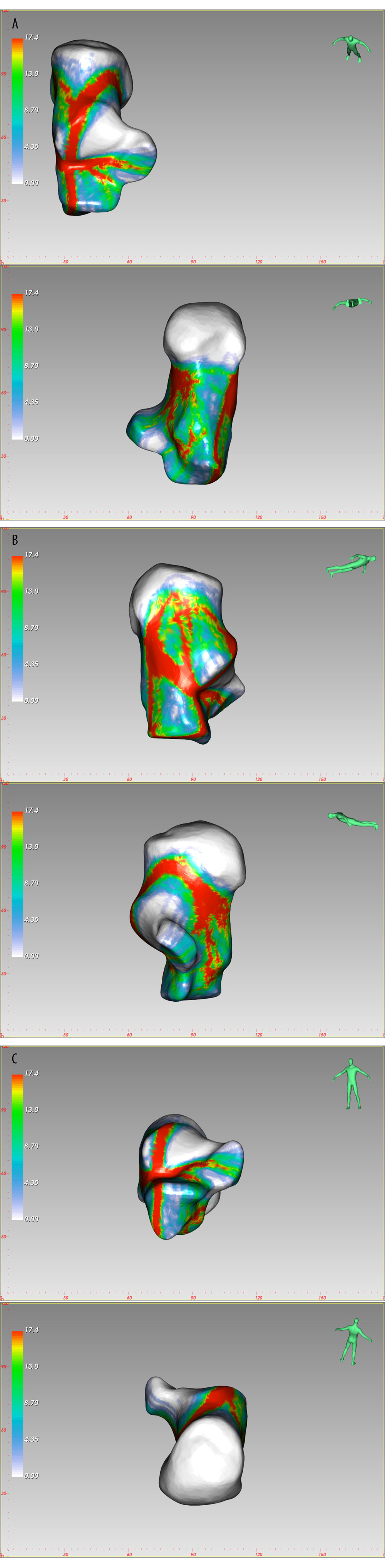 Figure 6. The fracture heatmap distribution of Sanders type 2A joint depression fracture, created by E-3D Medical 18.01 software (Central South University, Changsha, China). (A) Top view, Bottom view, (B) Lateral view, Medial view, (C) Front view, Rear view.
 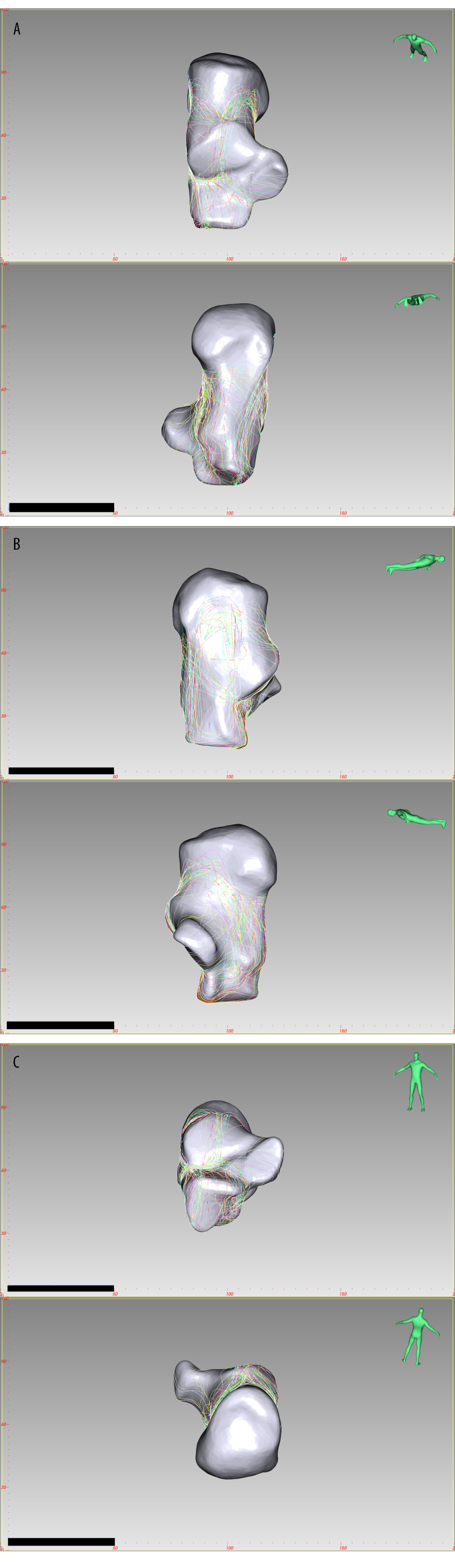 Figure 7. The fracture line distribution of Sanders type 2B joint depression fracture, created by E-3D Medical 18.01 software (Central South University, Changsha, China). (A) Top view, Bottom view, (B) Lateral view, Medial view, (C) Front view, Rear view.
 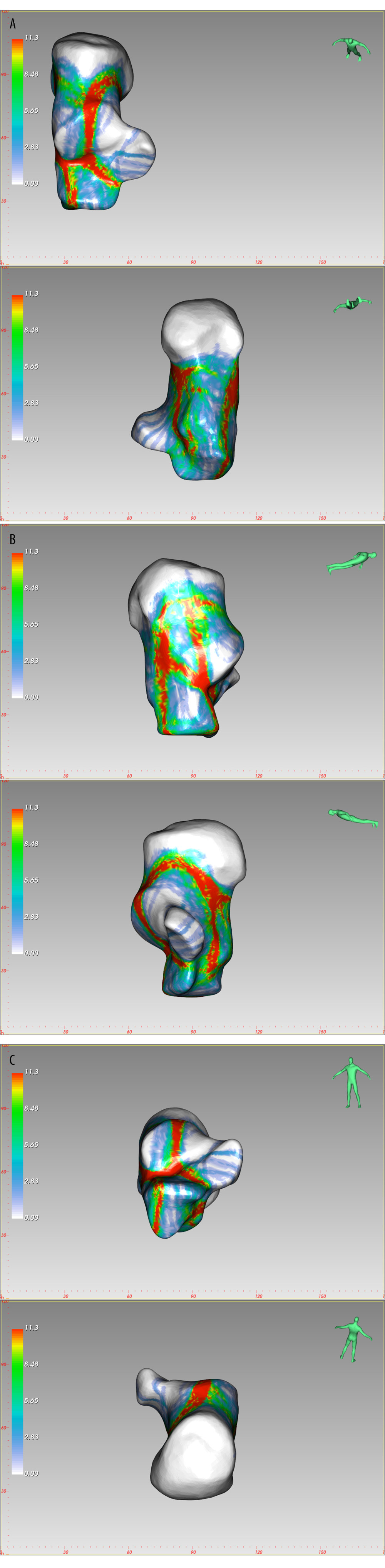 Figure 8. The fracture heatmap distribution of Sanders type 2B joint depression fracture, created by E-3D Medical 18.01 software (Central South University, Changsha, China). (A) Top view, Bottom view, (B) Lateral view, Medial view, (C) Front view, Rear view.
 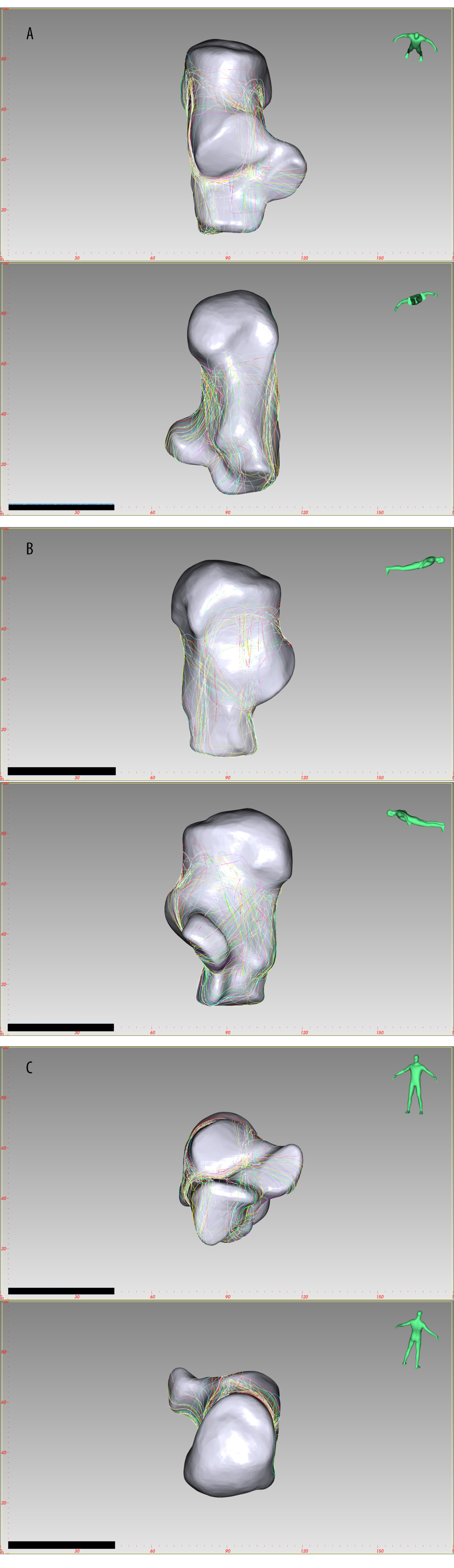 Figure 9. The fracture line distribution of Sanders type 2C joint depression fracture, created by E-3D Medical 18.01 software (Central South University, Changsha, China). (A) Top view, Bottom view, (B) Lateral view, Medial view, (C) Front view, Rear view.
 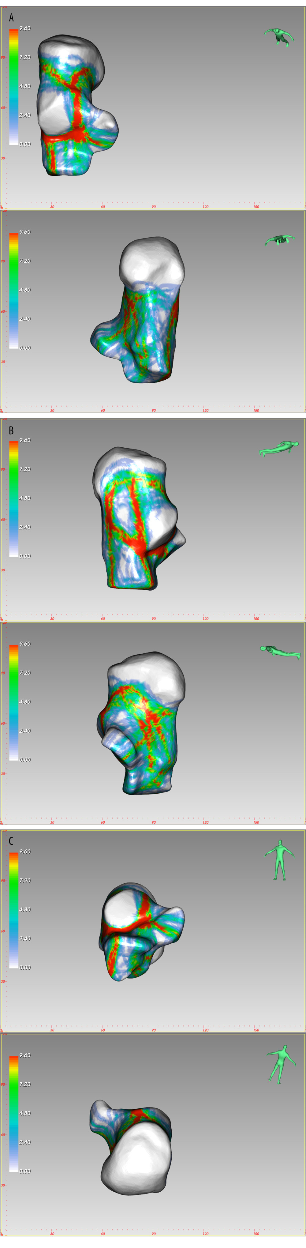 Figure 10. The fracture heatmap distribution of Sanders type 2C joint depression fracture, created by E-3D Medical 18.01 software (Central South University, Changsha, China). (A) Top view, Bottom view, (B) Lateral view, Medial view, (C) Front view, Rear view.
 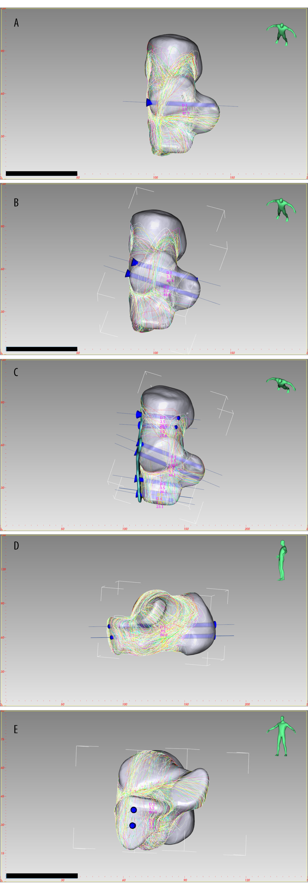 Figure 11. Optimal screw distribution in Sanders type 2A (A), Sanders type 2B (B) and Sanders type 2C (C) joint depression fracture. Optimal screw distribution in joint depression fracture (D, E) Medial view, Rear view. Created by E-3D Medical 18.01 software (Central South University, Changsha, China).
 References
1. Buckley RE, Tough S, Displaced intra-articular calcaneal fractures: J Am Acad Orthop Surg, 2004; 12(3); 172-78
2. Potter MQ, Nunley JA, Long-term functional outcomes after operative treatment for intra-articular fractures of the calcaneus: J Bone Joint Surg Am, 2009; 91(8); 1854-60
3. Marouby S, Cellier N, Mares O, Percutaneous arthroscopic calcaneal osteosynthesis for displaced intra-articular calcaneal fractures: Systematic review and surgical technique: Foot Ankle Surg, 2020; 26(5); 503-8
4. Gavlik JM, Rammelt S, Zwipp H, The use of subtalar arthroscopy in open reduction and internal fixation of intra-articular calcaneal fractures: Injury, 2002; 33(1); 63-71
5. Essex-Lopresti P, The mechanism, reduction technique, and results in fractures of the os calcis: Br J Surg, 1952; 39(157); 395-419
6. Sanders R, Fortin P, DiPasquale T, Walling A, Operative treatment in 120 displaced intraarticular calcaneal fractures. Results using a prognostic computed tomography scan classification: Clin Orthop Relat Res, 1993(290); 87-95
7. Vosoughi AR, Borazjani R, Ghasemi N, Different types and epidemiological patterns of calcaneal fractures based on reviewing CT images of 957 fractures: Foot Ankle Surg, 2021 [Online ahead of print]
8. Aghnia Farda N, Lai JY, Wang JC, Sanders classification of calcaneal fractures in CT images with deep learning and differential data augmentation techniques: Injury, 2021; 52(3); 616-24
9. Armitage BM, Wijdicks CA, Tarkin IS, Mapping of scapular fractures with three-dimensional computed tomography: J Bone Joint Surg Am, 2009; 91(9); 2222-28
10. Ni M, Lv ML, Sun W, Fracture mapping of complex intra-articular calcaneal fractures: Ann Transl Med, 2021; 9(4); 333
11. Su Q, Zhang Y, Liao S, 3D computed tomography mapping of thoracolumbar vertebrae fractures: Med Sci Monit, 2019; 25; 2802-10
12. Xie X, Zhan Y, Dong M, Two and three-dimensional CT mapping of Hoffa fractures: J Bone Joint Surg Am, 2017; 99(21); 1866-74
13. Franke J, von Recum J, Wendl K, Grutzner PAIntraoperative 3-dimensional imaging – beneficial or necessary?: Unfallchirurg, 2013; 116(2); 185-90 [in German]
14. Badillo K, Pacheco JA, Padua SO, Multidetector CT evaluation of calcaneal fractures: Radiographics, 2011; 31(1); 81-92
15. Halai M, Hester T, Buckley RE, Does 3D CT reconstruction help the surgeon to preoperatively assess calcaneal fractures?: Foot (Edinb), 2020; 43; 101659
16. Geerling J, Kendoff D, Citak M, Intraoperative 3D imaging in calcaneal fracture care-clinical implications and decision making: J Trauma, 2009; 66(3); 768-73
17. Cole PA, Mehrle RK, Bhandari M, Zlowodzki M, The pilon map: Fracture lines and comminution zones in OTA/AO type 43C3 pilon fractures: J Orthop Trauma, 2013; 27(7); e152-56
18. Mellema JJ, Doornberg JN, Dyer GS, Ring D, Distribution of coronoid fracture lines by specific patterns of traumatic elbow instability: J Hand Surg Am, 2014; 39(10); 2041-46
19. Mellema JJ, Doornberg JN, Molenaars RJ, Tibial plateau fracture characteristics: Reliability and diagnostic accuracy: J Orthop Trauma, 2016; 30(5); e144-51
20. Mellema JJ, Eygendaal D, van Dijk CN, Fracture mapping of displaced partial articular fractures of the radial head. J Shoulder Elbow Surg, 2016; 25(9); 1509-16
21. Li M, Li ZR, Li JT, Three-dimensional mapping of intertrochanteric fracture lines, 2019; 132(21); 2524-33
22. Yang Y, Yi M, Zou C, Mapping of 238 quadrilateral plate fractures with three-dimensional computed tomography: Injury, 2018; 49(7); 1307-12
23. Yang Y, Zou C, Fang Y, Mapping of both column acetabular fractures with three-dimensional computed tomography and implications on surgical management: BMC Musculoskelet Disord, 2019; 20(1); 255
24. Su QH, Liu J, Zhang Y, Three-dimensional computed tomography mapping of posterior malleolar fractures: World J Clin Cases, 2020; 8(1); 29-37
25. Lee P, Hunter TB, Taljanovic M, Musculoskeletal colloquialisms: How did we come up with these names?: Radiographics, 2004; 24(4); 1009-27
26. Pinto A, Brunese L, Pinto F, E-learning and education in radiology: Eur J Radiol, 2011; 78(3); 368-71
27. Ierardi AM, Xhepa G, Duka E, Ethylene-vinyl alcohol polymer trans-arterial embolization in emergency peripheral active bleeding: initial experience: Int Angiol, 2015; 34(6 Suppl 1); 28-35
28. Pinto A, Reginelli A, Pinto F, Errors in imaging patients in the emergency setting: Br J Radiol, 2016; 89(1061); 20150914
29. Grassi R, Lombardi G, Reginelli A, Coccygeal movement: Assessment with dynamic MRI: Eur J Radiol, 2007; 61(3); 473-479
30. Teubner E, Gerstenberger F, Walter BPathomechanical aspects of intra-articular calcaneus fractures. Typing, grading and surgical therapy: Aktuelle Traumatol, 1992; 22(6); 243-50 [in German]
31. Zwipp H, Rammelt S, Barthel SFracture of the calcaneus: Unfallchirurg, 2005; 108(9); 737-47 [in German]
32. Tsubone T, Toba N, Tomoki U, Prediction of fracture lines of the calcaneus using a three-dimensional finite element model: J Orthop Res, 2019; 37(2); 483-89
33. Meinberg EG, Agel J, Roberts CS, Fracture and dislocation classification compendium – 2018: J Orthop Trauma, 2018; 32(Suppl 1); S1-170
34. Veltman ES, van den Bekerom MP, Doornberg JN, Three-dimensional computed tomography is not indicated for the classification and characterization of calcaneal fractures: Injury, 2014; 45(7); 1117-20
35. Harnroongroj T, Jiamamornrat S, Tharmviboonsri T, Characteristics of anterior inferior calcaneal cortex: Foot Ankle Surg, 2019; 25(3); 323-26
36. Gatha M, Pedersen B, Buckley R, Fractures of the sustentaculum tali of the calcaneus: A case report: Foot Ankle Int, 2008; 29(2); 237-40
37. Gras F, Marintschev I, Wilharm ASustentaculum tali screw placement for calcaneus fractures – different navigation procedures compared to the conventional technique: Z Orthop Unfall, 2010; 148(3); 309-18 [in German]
Figures
Figure 1. Flow charts of the calcaneal fracture map. (A) The segment and split functions were used to create each calcaneal fracture fragment by Mimics Research 20.0 (Materialise, Leuven, Belgium) software. (B) The calcaneal fracture fragments were reduced in 3-matic Research 12.0 (Materialise, Leuven, Belgium) software. (C) In the E-3D Medical 18.01(Central South University, Changsha, China) software, after superimposing the fractured calcaneus entity with the calcaneus template, draw the fracture line on the template.Figure 2. The division of the anterior part of calcaneus (APC) and middle talar articular surface. (A) Top view, (B) Front view.Figure 3. The fracture line distribution of Sanders type 2 joint depression fracture, created by E-3D Medical 18.01 software (Central South University, Changsha, China). (A) Top view, Bottom view, (B) Lateral view, Medial view, (C) Front view, Rear view.Figure 4. The fracture heatmap distribution of Sanders type 2 joint depression fracture, created by E-3D Medical 18.01 software (Central South University, Changsha, China). (A) Top view, Bottom view, (B) Lateral view, Medial view, (C) Front view, Rear view.Figure 5. The fracture line distribution of Sanders type 2A joint depression fracture, created by E-3D Medical 18.01 software (Central South University, Changsha, China). (A) Top view, Bottom view, (B) Lateral view, Medial view, (C) Front view, Rear view.Figure 6. The fracture heatmap distribution of Sanders type 2A joint depression fracture, created by E-3D Medical 18.01 software (Central South University, Changsha, China). (A) Top view, Bottom view, (B) Lateral view, Medial view, (C) Front view, Rear view.Figure 7. The fracture line distribution of Sanders type 2B joint depression fracture, created by E-3D Medical 18.01 software (Central South University, Changsha, China). (A) Top view, Bottom view, (B) Lateral view, Medial view, (C) Front view, Rear view.Figure 8. The fracture heatmap distribution of Sanders type 2B joint depression fracture, created by E-3D Medical 18.01 software (Central South University, Changsha, China). (A) Top view, Bottom view, (B) Lateral view, Medial view, (C) Front view, Rear view.Figure 9. The fracture line distribution of Sanders type 2C joint depression fracture, created by E-3D Medical 18.01 software (Central South University, Changsha, China). (A) Top view, Bottom view, (B) Lateral view, Medial view, (C) Front view, Rear view.Figure 10. The fracture heatmap distribution of Sanders type 2C joint depression fracture, created by E-3D Medical 18.01 software (Central South University, Changsha, China). (A) Top view, Bottom view, (B) Lateral view, Medial view, (C) Front view, Rear view.Figure 11. Optimal screw distribution in Sanders type 2A (A), Sanders type 2B (B) and Sanders type 2C (C) joint depression fracture. Optimal screw distribution in joint depression fracture (D, E) Medial view, Rear view. Created by E-3D Medical 18.01 software (Central South University, Changsha, China). Tables
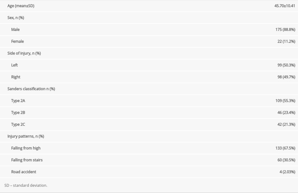 Table 1. Patient demographics and calcaneal fracture characteristics (n=197).
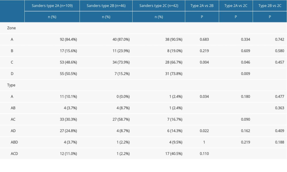 Table 2. Fracture distribution in APC and middle talar articular surface (N=197).Table 1. Patient demographics and calcaneal fracture characteristics (n=197).Table 2. Fracture distribution in APC and middle talar articular surface (N=197).
 In Press
Clinical Research
Comparative Effectiveness of a Nurse-Led Care Model vs Usual Care in Rheumatoid Arthritis: A Longitudinal C...Med Sci Monit In Press; DOI: 10.12659/MSM.953211
Clinical Research
Impact of Treatment Modality on Pain, Sexual Function, and Psychological Well-Being in Patients With Bartho...Med Sci Monit In Press; DOI: 10.12659/MSM.952422
Clinical Research
Association Between Radiographic Knee Osteoarthritis, Pre-Fracture Mobility, and Hip Fracture Patterns in O...Med Sci Monit In Press; DOI: 10.12659/MSM.952678
Clinical Research
Association Between Total Cholesterol–to–High-Density Lipoprotein Ratio and Gestational Hypertension: A Cas...Med Sci Monit In Press; DOI: 10.12659/MSM.952395
Most Viewed Current Articles
17 Jan 2024 : Review article 14,176,084
Vaccination Guidelines for Pregnant Women: Addressing COVID-19 and the Omicron VariantDOI :10.12659/MSM.942799
Med Sci Monit 2024; 30:e942799
13 Nov 2021 : Clinical Research 3,757,530
Acceptance of COVID-19 Vaccination and Its Associated Factors Among Cancer Patients Attending the Oncology ...DOI :10.12659/MSM.932788
Med Sci Monit 2021; 27:e932788
14 Dec 2022 : Clinical Research 2,466,116
Prevalence and Variability of Allergen-Specific Immunoglobulin E in Patients with Elevated Tryptase LevelsDOI :10.12659/MSM.937990
Med Sci Monit 2022; 28:e937990
16 May 2023 : Clinical Research 708,768
Electrophysiological Testing for an Auditory Processing Disorder and Reading Performance in 54 School Stude...DOI :10.12659/MSM.940387
Med Sci Monit 2023; 29:e940387